The Beginner’s Guide to Conditional Formatting in Google Sheets
If you’re looking to understand what conditional formatting is, how it works, and the ways you can use it in Google Sheets, this article is for you.
In this detailed guide, I’ll introduce you to the basics of conditional formatting in Google Sheets and how you can apply it to different data sets (large or small) to make them much easier to analyze.
Plus, I’ll share several examples and use cases to demonstrate the different conditional formatting options available in Google Sheets.
Sound interesting? Keep reading.
What Is Conditional Formatting?
Conditional formatting is a feature in Google Sheets with which you can highlight cells, columns, rows, or complete data sets with different colors and change their text style based on your pre-defined conditions.
The main benefit of conditional formatting is that it allows you to instantly identify the values and information you’re looking for irrespective of the size of your data set.
For example, you have a Google Sheet that lists all your customers, project types, project managers, project deadlines, and statuses.
Let’s say you want to highlight the projects managed by Matthew, one of your project managers.
Instead of searching manually, you can apply a simple conditional formatting rule to highlight all the projects Matthew is managing.
Easy, isn’t it?
That’s a very simple example of conditional formatting.
You can do a lot more with it which we’ll see later in the post.
But first, let’s see how to apply conditional formatting to a data set.
Where to Find Conditional Formatting
Applying conditional formatting is pretty simple.
Here are the steps you need to follow.
Step 1: Open the Google Sheet that contains your data set.
Step 2: Click on Format→ Conditional Formatting in the top menu.
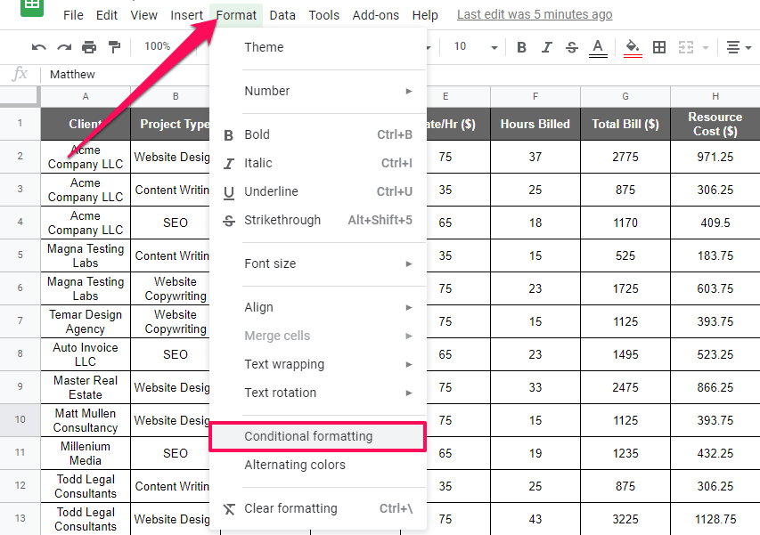
This opens the conditional formatting rules panel on the right of your screen.
There are three main options here using which you can apply different conditional formatting rules. I’ll give you their quick overview before explaining them in more detail in the next sections.
Apply To Range
This is where you select the cell range on which you want to apply conditional formatting. It can be a single cell, a row, a column, or a complete table.
Format Rules
This is where you apply if-then conditions and define the criteria based on which you want to highlight data and change its formatting. You can choose from a long list of pre-defined conditions or apply custom formulas for advanced conditional formatting.
Formatting Styles
This is where you select the color and the text style you want to use to highlight the data that meets your format rules.
Let’s see how all these options work together.
How Conditional Formatting Works In Google Sheets
Applying conditional formatting to your data involves several steps. In this section, I’ll describe each step in detail.
Step#1: Selecting Data Range
This is the first step of applying conditional formatting after you’ve opened the Google Sheet that contains your data.
Start by choosing the cells where you want to apply conditional formatting. For example, let’s apply conditional formatting to the Profit column in our sample sheet.
Click on the column and choose conditional formatting from the Format section.
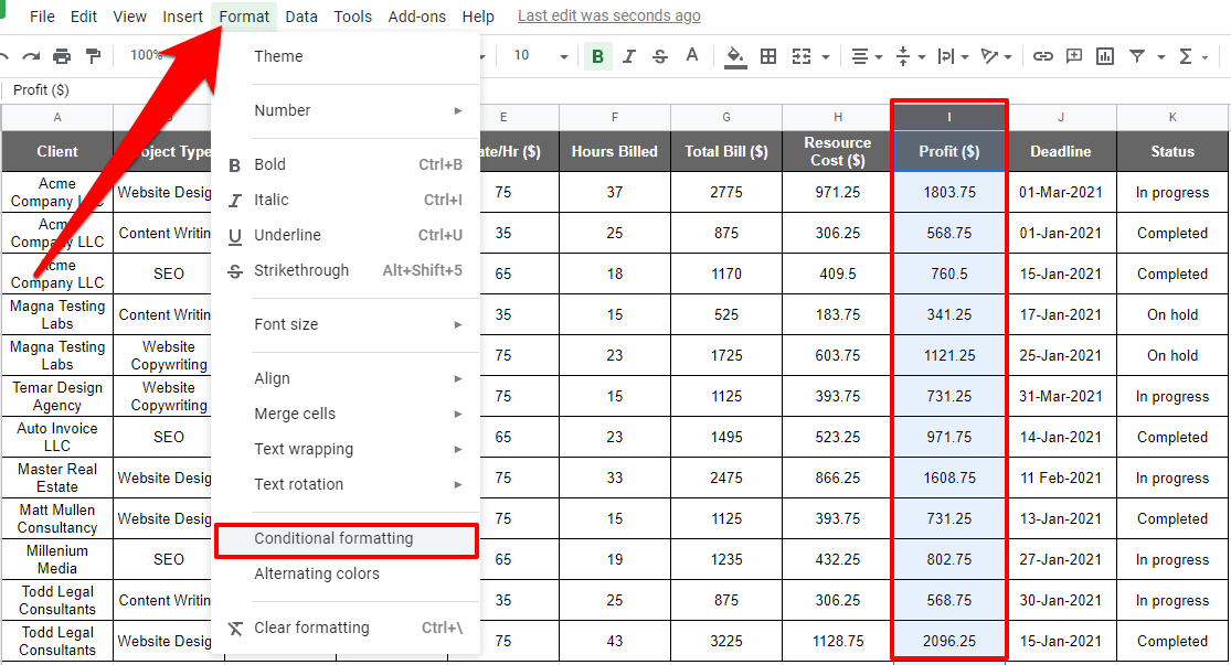
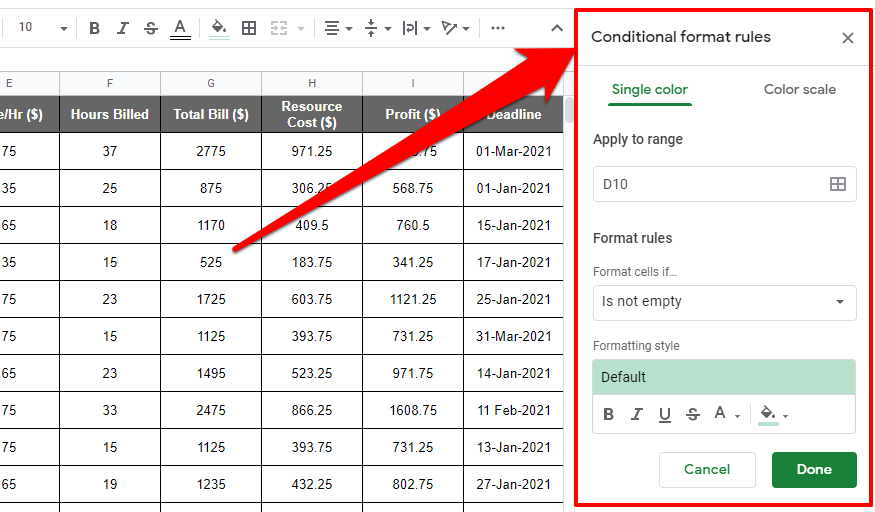
This will open the conditional formatting rules pane that shows your selected range.
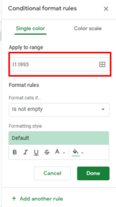
If you want to apply conditional formatting to another column in the same rule, click on the table icon under “Apply to Range.”
This will open the “Select a data range” pop-up. Click on the button to “Add another range” and choose the cells you want to add.
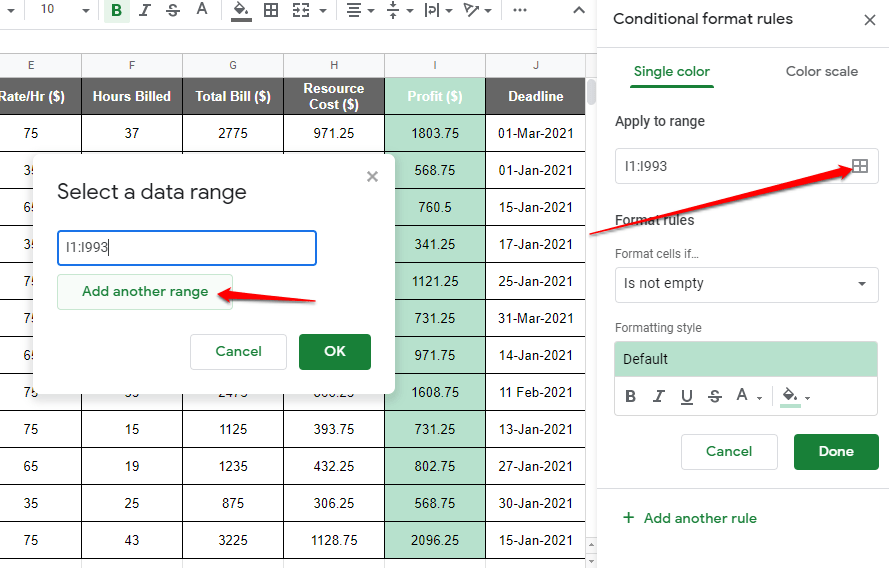
You’ll now have two separate data ranges.

Using this process, you can add as many cells or data ranges as you want.
The formatting rules that you choose in the next step will apply to all your data ranges.
Step#2: Creating Format Rules With If-Then Conditions
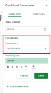
Format Rules are the conditions based on which Google Sheets will apply conditional formatting on your selected data range.
Once you’ve chosen your data, click on the dropdown menu in the conditional formatting rules section and choose the condition you want to apply.
Here are the different types of Format Rules you can choose from the list.
Cell Empty/Not Empty
In this condition, you can choose “Is empty” or “Is not empty” as formatting conditions.
For example, if you choose “Is empty” Google Sheets will apply conditional formatting to any cells in your data range that are empty.
Simple, right?
No cells will be highlighted if none of them are empty.
Cell Text
In this formatting rule, you can create conditions based on the text content of your selected cells.
You have five different options:
- Text Contains
- Text Does Not Contain
- Text Starts With
- Text Ends With
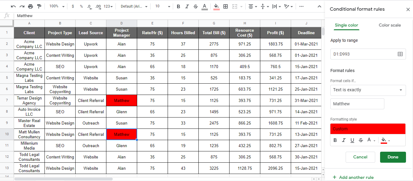
- Text Is Exactly
All these options are self-explanatory.
But let me describe just one of them.
Let’s say you apply conditional formatting to a data range and choose “Text Starts With.”
This opens up a text field where you can enter the text content you want Google Sheets to search for.

Any cells that start with the word Alan will be highlighted once you apply this formatting rule.
All the other text conditions work the same way.
Cell Date
In this formatting rule, you can highlight the cells in your data range based on their dates.
Here are your options.
- Date Is
- Date Is Before
- Date Is After
You can only apply this formatting rule to cells that contain dates in the right format.
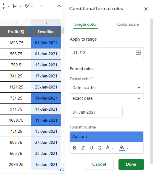
Let’s say you want to highlight the cells with dates before Jan 2021.
Choose “Date Is Before” from the dropdown list.
This shows you another dropdown.
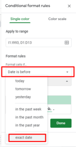
Choose “exact date” from this dropdown to open a text field. Enter the exact date to highlight all the cells before it.
In the same manner, you can use the other options from this list to highlight cells from a specific date or date range.
Cell Numerical Value
In this formatting rule, you can highlight the cells in your data range based on their numerical value.
You have plenty of options here
- Greater than
- Greater than or equal to
- Less than
- Less than or equal to
- Is equal to
- Is not equal to
- Is between
- Is not between
When you choose any of the options from this list, Google Sheets will highlight the cells that match your criteria.
For example, let’s say you want to highlight the projects that earned more than $1000 in profit.
Here’s how you’ll do it.
Choose the Profit column and in the Format Rule choose “Greater than”
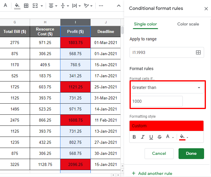
As you can see, choosing this option gives you a text field in which you can enter a numerical value.
In our example, I entered 1000 since I wanted to highlight the cells where the profit was more than $1000.
And as the screenshot shows, Google Sheets immediately highlighted the relevant cells.
But what if you want to highlight the cells with a different color? Or want to use different colors for every conditional formatting rule you apply?
Let me explain how to do it in the next section.
Using Formatting Styles To Highlight Data
This is where you configure the formatting style of the cells you want to highlight based on your format rules.
You can change the color and text style of the cells that meet your criteria.
Here’s how to do it.
Using Conditional Formatting to Change Cell Colors
You’ve chosen your data range and set up your format rules.
Now go to the Formatting Styles section and choose a color from the “Fill color” section to highlight cells.
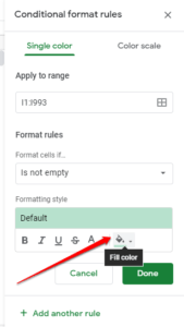
The default color in Google Sheets is light green but you can choose any color you want.
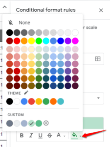
For demonstration, I’ve chosen the blue color from the list.
Here’s what the highlighted cells would look like.
Using Conditional Formatting To Apply Text Styles
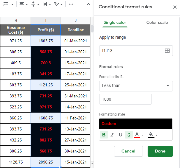
Let’s say you want to bold and strikethrough all the cells where the value is less than 1000, color them black, and change the text color to red.
Here’s how to do it.
Choose your data range, set your format rules, and choose the bold and strikethrough option under Formatting Style. Also, choose the black color from the Fill Color section and the red color from the text color section.
Here’s how the cells would appear now.
You can also apply different formatting styles and colors to cells highlighted for different conditional formatting rules.
Applying Formatting Styles To Multiple Conditional Formatting Rules
Add a new conditional formatting rule following the steps I described earlier.
Choose its data range and format rules.
Now finally go to the formatting style section and choose the colors and formatting styles you want.
Let’s say that in addition to the previous condition, we want to highlight the cells where Alan is the project manager.
Here’s how the highlighted cells will now appear.
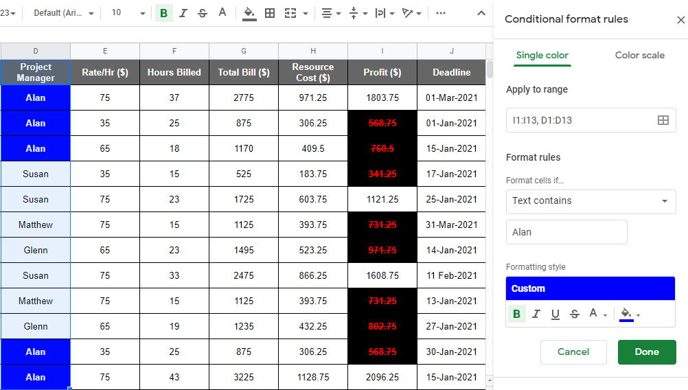
You can add as many data ranges as you want and highlight them using different formatting styles following these steps.
Conditional Formatting With Color Scale
Until now, I’ve described the process of conditional formatting with a single color which means that all the highlighted cells for a given condition will use the same color.
However, there’s another option for highlighting the cells that meet your criteria.
It’s called the color scale.
Using a color scale, you can highlight the values in your range using a color spectrum. The higher the value the darker the color (or vice versa).
It is ideal for highlighting numerical values like numbers or percentages to identify the highest, lowest, and mid-point values.
Here’s how to apply it.
Let’s say we want to apply the color scale on the Profit column in our table so that we can identify the most and the least profitable projects.
Choose the Profit column and click on Conditional Formatting from the Format menu.
Now choose “Color scale” in the conditional formatting rules.
You can choose a color spectrum from the default list or set your own colors for the minimum and maximum values.
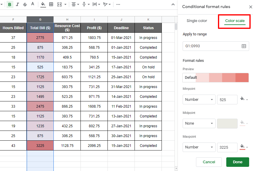
Choose the relevant value type for the Minpoint and Maxpoint fields. In our example, the values are numbers. But you can also apply the color scale to percentage values.
How To Remove Conditional Formatting
Once you’ve applied conditional formatting to a data range, a cell or a column, it will remain in place until you remove it.
How do you remove conditional formatting from a data set?
Just follow the simple steps below.
Step#1: Close the conditional formatting rules pane if it’s open in your Google Sheet.
Step#2: Now click on any cell where you’ve applied conditional formatting
Step#3: Click on Format→ Conditional Formatting
Step#4: This will open the conditional formatting rules pane but instead of the setup section, you’ll see the list of active rules in your sheet.
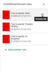
Step#5: Every rule has a delete icon next to it.
Step#6: Click the delete icon next to any conditional formatting rules that you want to remove.
That’s it, you’ve successfully removed conditional formatting from the selected cells.
When you remove a rule, the cells highlighted because of it go back to their default colors.
Are You Ready To Use Conditional Formatting In Google Sheets?
I’ve covered all the fundamentals of conditional formatting in this article using which you can easily highlight your desired values/cells in any data set.
However, there’s a lot more to conditional formatting (like custom conditions and advanced rules) that I did not discuss here since this was a beginner’s guide.
Here’s my suggestion.
Create a dummy data set and apply different conditional formatting rules to it to get a better understanding of how it works.
Once you’re proficient enough with the basic conditions, you can move to the more advanced and complex rules later.
Let me know if you have questions in the comments section.